Long Tails

Long tails refer to small numbers of samples which occur a large number of times. When we plot these out, they form a small sliver far to the right of the center of mass which looks like a tail. They indicate the presence of outliers whose unusual behaviors may be of interest to us.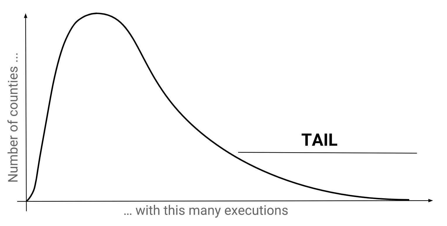 In context of Texas executions, the long tail refers to a small number of counties which have been known to conduct a large number of executions.

Let’s find the percentage of executions from each county so that we can pick out the ones in the tail.

As will become increasingly evident, the shape of the tables tell us a lot about the operations we need to perform. (This is analogous to dimensional analysis in physics.) In this case, we can discern that the methods we’ve covered so far are inadequate: The Beazley chapter dealt with individual rows of data, but it’s clear that we need to do some aggregation to find county-level data. The Claims of Innocence chapter taught us aggregation, but those functions would end up aggregating the dataset into one row when we really want one row per county.

The GROUP BY Block

This is where the GROUP BY block comes in. It allows us to split up the dataset and apply aggregate functions within each group, resulting in one row per group. Its most basic form is GROUP BY <column>, <column>, ... and comes after the WHERE block.

If you recall A Strange Query, alarm bells would be going off in your head. Didn’t we just learn not to mix aggregated and non-aggregated columns? The difference here is that grouping columns are the only columns allowed to be non-aggregate. After all, all the rows in that group must have the same values on those columns so there’s no ambiguity in the value that should be returned.

You may have also noticed our use of AS. It’s what we call “aliasing”. In the SELECT block, <expression> AS <alias> provides an alias that can be referred to later in the query. This saves us from rewriting long expressions, and allows us to clarify the purpose of the expression.

The HAVING Block

This next exercise illustrates that filtering via the WHERE block happens before grouping and aggregation. This is reflected in the order of syntax since the WHERE block always precedes the GROUP BY block.

This is all good but what happens if we want to filter on the result of the grouping and aggregation? Surely we can’t jump forward into the future and grab information from there. To solve this problem, we use HAVING.

Practice

This quiz is designed to challenge your understanding. Read the explanations even if you get everything correct.

Nested Queries

Now, you may ask, wouldn’t we be done if we could just run something like this?

SELECT
  county,
  PERCENT_COUNT(*)
FROM executions
GROUP BY county

Percentages are such a common metric—shouldn’t such a function exist? Unfortunately not, and perhaps for good reason: Such a function would need to aggregate both within the groups (to get the numerator) and throughout the dataset (to get the denominator). But each query either has a GROUP BY block or doesn’t. So what we really need are two separate queries, one which aggregates with a GROUP BY and another that aggregates without. We can then combine them using a technique called “nesting”.

Here’s an example of how nesting works. The parentheses are important for demarcating the boundary between the inner query and the outer one:

To reiterate, nesting is necessary here because in the WHERE clause, as the computer is inspecting a row to decide if its last statement is the right length, it can’t look outside to figure out the maximum length across the entire dataset. We have to find the maximum length separately and feed it into the clause. Now let’s apply the same concept to find the percentage of executions from each county.

I’ve quietly slipped in an ORDER BY block. Its format is ORDER BY <column>, <column>, ... and it can be modified by appending DESC if you don’t want the default ascending order.

Harris County

Is it surprising that Harris (home to the city of Houston), Dallas, Bexar and Tarrant account for about 50% of all executions in Texas? Perhaps it is, especially if we start from the assumption that executions should be distributed evenly across counties. But a better first approximation is that executions are distributed in line with the population distribution. The 2010 Texas Census shows that the 4 counties had a population of 10.0M which is 40.0% the population of Texas (25.1M). This makes the finding slightly less surprising.

But breaking this tail down further, we realize that Harris county accounts for most of the delta. It only has 16.4% of the population, but 23.1% of the executions. That’s almost 50% more than it’s supposed to have.

Numerous studies have examined why Harris county has been so prolific and several factors have been suggested:

• Prosecutions have been organized and well-financed, while defenses have been court-financed and poorly-incentivized. (Source, see p49)

• The long-time district attorney was determined and enthusiastic about the death penalty.

• Judges in Texas are elected, and the population has supported the death penalty. (Source)

• Checks and balances in the Harris county judicial system have not worked. (Source, see p929)

Recap

In this section, we’ve learned to aggregate over groups and to use nesting to use the output of an inner query in an outer one. These techniques have the very practical benefit of allowing us to calculate percentages.

In the next chapter, we’ll learn about JOINs which will enable us to work with multiple tables.