Hiatuses

This graph shows executions over time.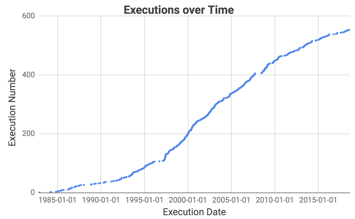 Notice that there have been several extended periods when no executions took place. Our goal is to figure out exactly when they were and research their causes.

Our strategy is to get the table into a state where each row also contains the date of the execution before it. We can then find the time difference between the two dates, order them in descending order, and read off the longest hiatuses.

Thinking about Joins

None of the techniques we’ve learned so far are adequate here. Our desired table has the same length as the original executions table, so we can rule out aggregations which produce a smaller table. The Beazley chapter only taught us row operations which limit us to working with information already in the rows. However, the date of the previous execution lies outside a row so we have to use JOIN to bring in the additional information.

Let’s suppose the additional information we want exists in a table called previous which has two columns (ex_number, last_ex_date). We would be able to run the following query to complete our task:

SELECT
  last_ex_date AS start,
  ex_date AS end,
  ex_date - last_ex_date AS day_difference
FROM executions
JOIN previous
  ON executions.ex_number = previous.ex_number
ORDER BY day_difference DESC
LIMIT 10

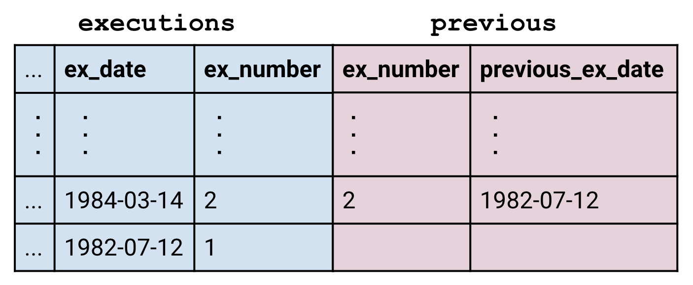
The JOIN block is the focus of this section. Instead of viewing it as a line on its own, it is often helpful to look at it like this: This emphasizes how JOIN creates a big combined table which is then fed into the FROM block just like any other table.

Types of Joins

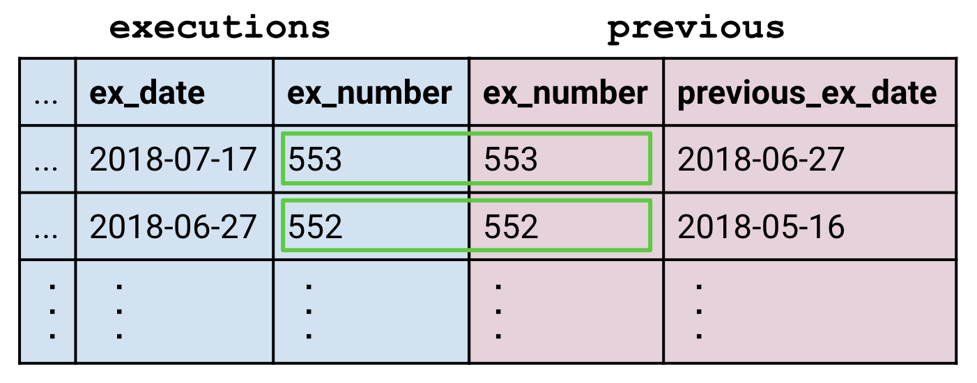
The JOIN block takes the form of <table1> JOIN <table2> ON <clause>. The clause works the same way as in WHERE <clause>. That is, it is a statement that evaluates to true or false, and anytime a row from the first table and another from the second line up with the clause being true, the two are matched:

But what happens to rows which have no matches? In this case, the previous table didn’t have a row for execution number 1 because there aren’t any executions prior to it.

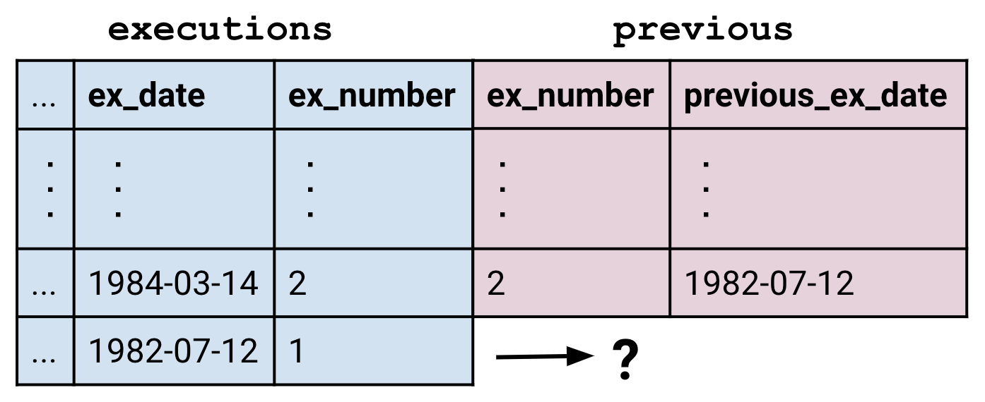
The JOIN command defaults to performing what is called an “inner join” in which unmatched rows are dropped.

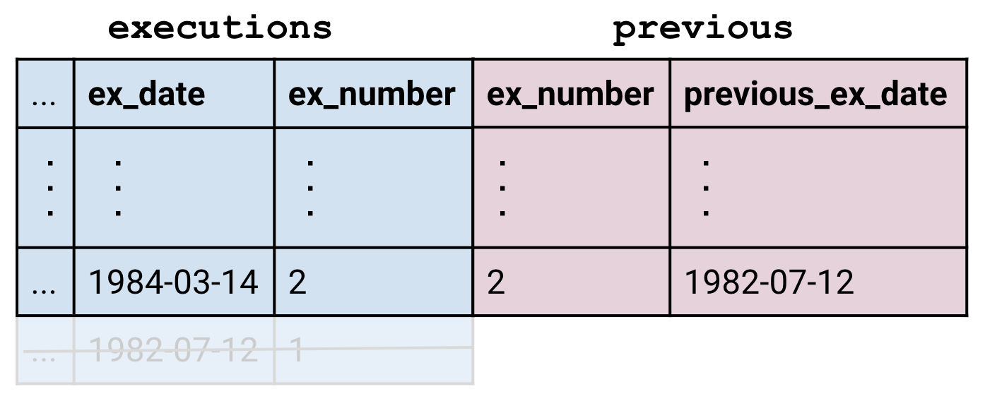
To preserve all the rows of the left table, we use a LEFT JOIN in place of the vanilla JOIN. The empty parts of the row are left alone, which means they evaluate to NULL.

The RIGHT JOIN can be used to preserve unmatched rows in the right table, and the OUTER JOIN can be used to preserve unmatched rows in both.

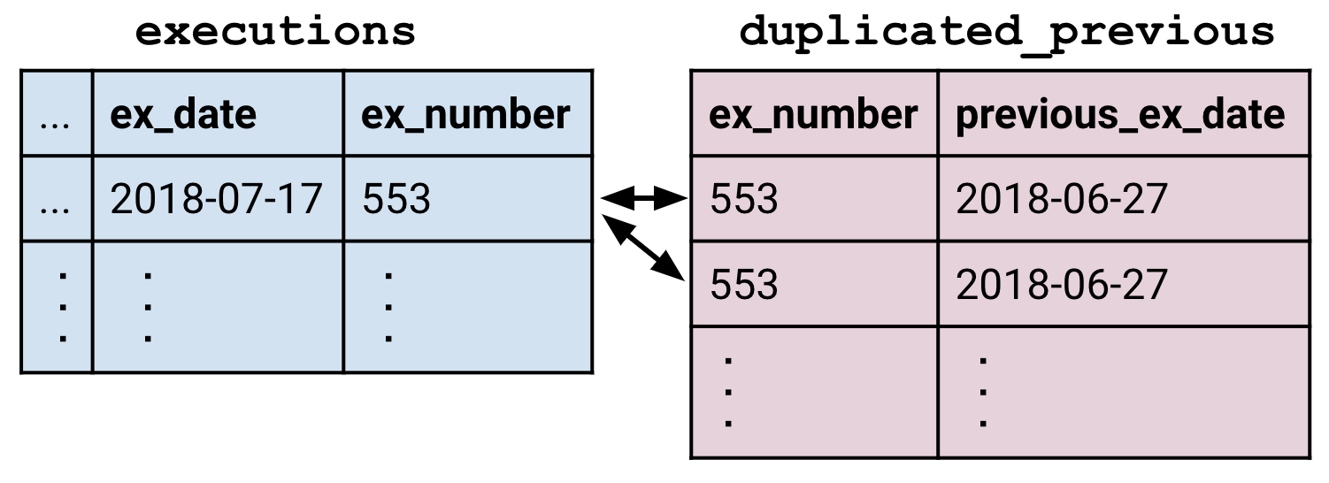
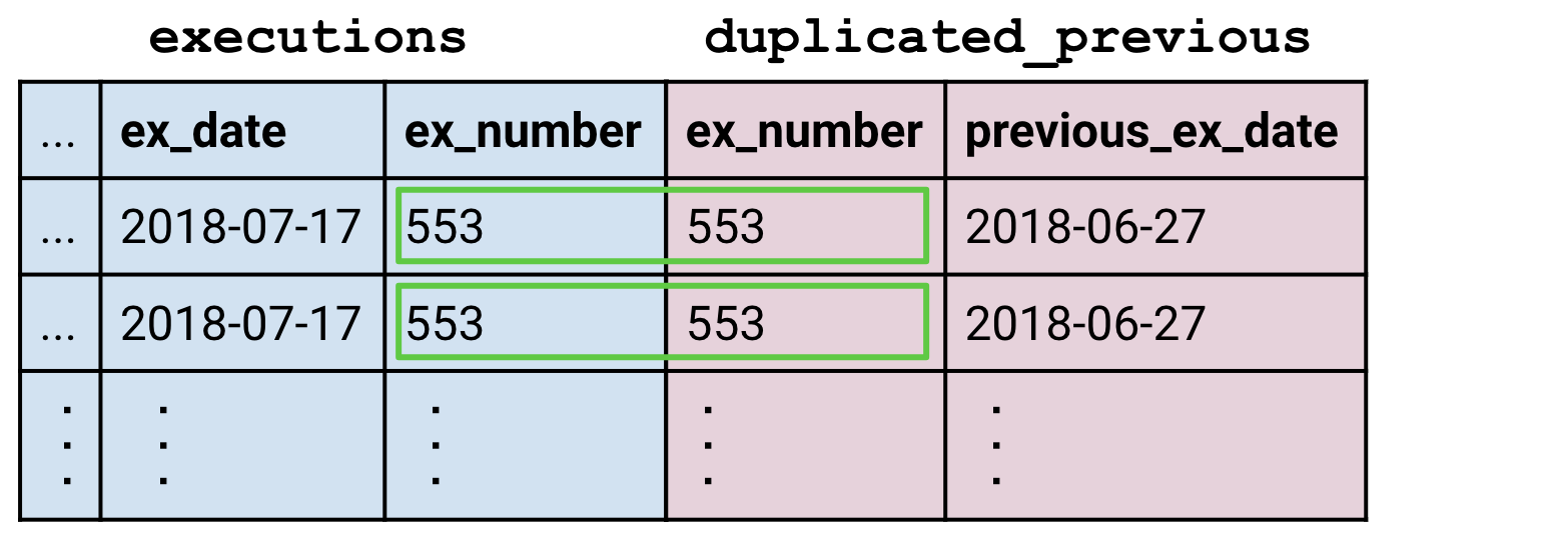
The final subtlety is handling multiple matches. Say we have a duplicated_previous table which contains two copies of each row of the previous table. Each row of executions now matches two rows in duplicated_previous. The join creates enough rows of executions so that each matching row of duplicated_previous gets its own partner. In this way, joins can create tables that are larger than their constituents.

Dates

Let’s take a break from joins for a bit and look at this line in our template query:

  ex_date - last_ex_date AS day_difference

We’ve made a big assumption that we can subtract dates from one another. But imagine you’re the computer receiving a line like this. Do you return the number of days between the dates? Why not hours or seconds? To make things worse, SQLite doesn’t actually have date or time types (unlike most other SQL dialects) so the ex_date and last_ex_date columns look like ordinary strings to you. You’re effectively being asked to do 'hello' - 'world'. What does that even mean?

Fortunately, SQLite contains a bunch of functions to tell the computer: “Hey, these strings that I’m passing you actually contain dates or times. Act on them as you would a date.”

Self Joins

With what we learned about dates, we can correct our template query:

SELECT
  last_ex_date AS start,
  ex_date AS end,
  JULIANDAY(ex_date) - JULIANDAY(last_ex_date)
    AS day_difference
FROM executions
JOIN previous
  ON executions.ex_number = previous.ex_number
ORDER BY day_difference DESC
LIMIT 5

The next step is to build out the previous table.

Now we can nest this query into our template above:

previous is derived from executions, so we’re effectively joining executions to itself. This is called a “self join” and is a powerful technique for allowing rows to get information from other parts of the same table.

We’ve created the previous table to clarify the purpose that it serves. But we can actually write the query more elegantly by joining the executions table directly to itself.

We can now use the precise dates of the hiatuses to research what happened over each period. In the years immediately after the ban on capital punishment was lifted, there were long periods without executions due to the low number of death sentences, coupled with legal challenges to the new ruling. We thus exclude intermissions before 1993 and focus on two major hiatuses since.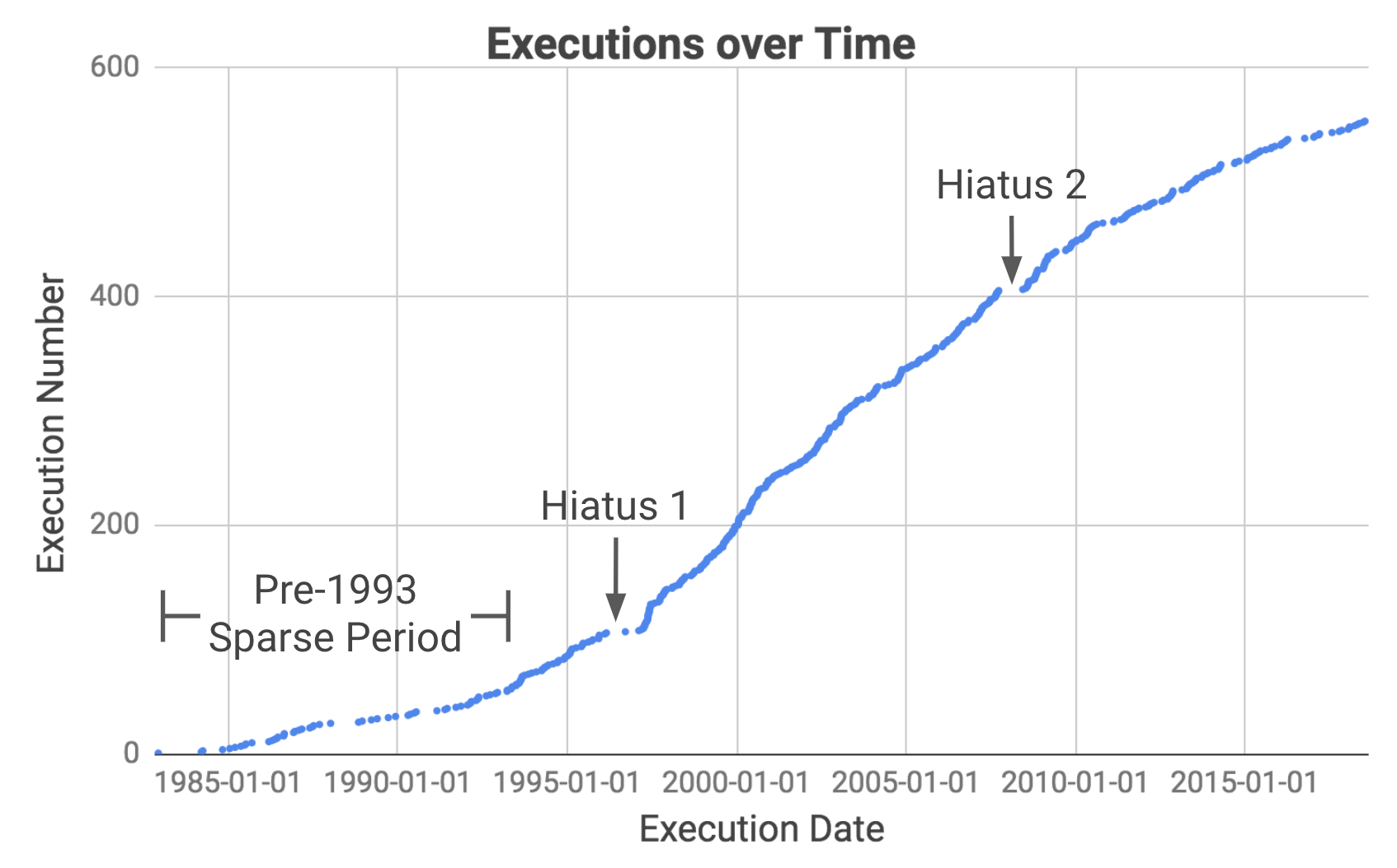

Hiatus 1 was due to legal challenges to the Antiterrorism and Effective Death Penalty Act of 1996 created in response to the 1993 World Trade Center and 1995 Oklahoma City bombings. The act limited the appeals process to make the death penalty more effective especially for terrorism cases (Source).

Hiatus 2 was caused by a stay enacted by the Supreme Court while it weighed in on Baze v. Rees which examined if lethal injection violates the Eighth Amendment prohibiting “cruel and unusual punishment”. This affected executions across America because most states were using the same drug cocktail as Kentucky. The Supreme Court eventually affirmed the Kentucky court decision and executions in Texas resumed a few months later.

Recap

The big idea behind JOINs has been to create an augmented table because the original didn’t contain the information we needed. This is a powerful concept because it frees us from the limitations of a single table and allows us to combine multiple tables in potentially complex ways. We’ve also seen that with this extra complexity, meticulous bookkeeping becomes important. Aliasing tables, renaming columns and defining good JOIN ON clauses are all techniques that help us maintain order.